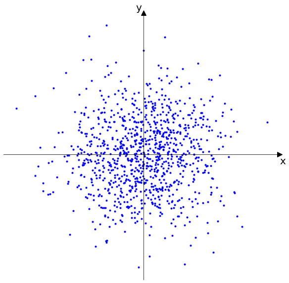
Distribution of landing spots
The probability density function (PDF) for the normal distribution is given by the following (somewhat intimidating) formula: $$ f(x) = \frac{1}{\sigma \sqrt{2\pi}} e^{-\frac{1}{2} \lparen \frac{x - \mu}{\sigma} \rparen^2} $$
It describes the well-known bell-shaped curve that is centered around the mean \(\mu\), has inflection points at one standard deviation \(\sigma\) around the mean, and integrates to one. Because of the central limit theorem, this curve is lurking behind every corner in statistics.
I recently read three beautiful derivations of this function in Jaynes (2003). Here I'm expanding on the Herschel-Maxwell derivation, following the steps of this video. I'm starting off with a thought experiment given by Herschel himself in 1869:
Suppose a ball dropped from a given height, with the intention that it shall fall on a given mark.1
Imagine we repated this little experiment a thousand times.
We might end up with something like this:
Distribution of landing spots
Each dot represents a landing spot of the dropped ball. I drew a Cartesian coordinate system over the dots whose origin represents the mark we aimed for with the ball. The values of \(x\) and \(y\) of a point are the error in the respective direction (how far off the landing position is from the origin). Now we are looking for the joint probability distribution \(p(x, y)\).
Herschel makes two postulates about this joint distribution:2
Combining both postulates leads us to an equation that relates \(x\) and \(y\) to the square root of the sum of their squares via two different functions. $$ f(x) \cdot f(y) = g(\sqrt{x^2 + y^2}) $$
However, by setting \(y = 0\) we see that one function can be expressed in terms of the other \(f(x)f(0) = g(x)\). Thus we can rewrite the previous equation with only one function. After substituting \(f(\sqrt{x^2 + y^2})f(0)\) for \(g(\sqrt{x^2 + y^2})\) and dividing both sides by \(f(0)^2\) we get $$ \frac{f(x)}{f(0)} \cdot \frac{f(y)}{f(0)} = \frac{f(\sqrt{x^2 + y^2})}{f(0)} $$
To make the next steps more obvious, we substitute \(h(x) = \frac{f(x)}{f(0)}\). $$ h(x) \cdot h(y) = h(\sqrt{x^2 + y^2}) $$
Clearly \(h(x)\) is a composition of the square and an exponential function. The base of the exponential doesn't matter, the important point is the relationship \(b^x \cdot b^y = b^{x+y}\). Since \(b^x = \lparen c^{\log_c b}\rparen^x = c^{(\log_c b) x}\), we can just pick a base and introduce a constant \(a\) that allows us to switch to any base: \(h(x) = e^{ax^2}\). After expanding \(h(x)\) again, we solve for \(f(x)\). $$ f(x) = f(0) \cdot e^{ax^2} $$
We know that \(x^2\) is always positive and we know that the exponential function grows indefinitely for positive values of \(x\). However, we want to derive a probability distribution, so \(a\) must be less than zero: \(a = - (b^2)\). \(f(0)\) is some constant that we will call \(c\). $$ f(x) = c \cdot e^{-(b^2)x^2} $$
Now the maximum of each function \(f(x)\) is at \(x = 0\) and the functions are symmetric around their maximum.
Our formula describes a family of bell-shaped functions.
Composing basic functions: only negative values of \(a\) yield bell-shaped functions.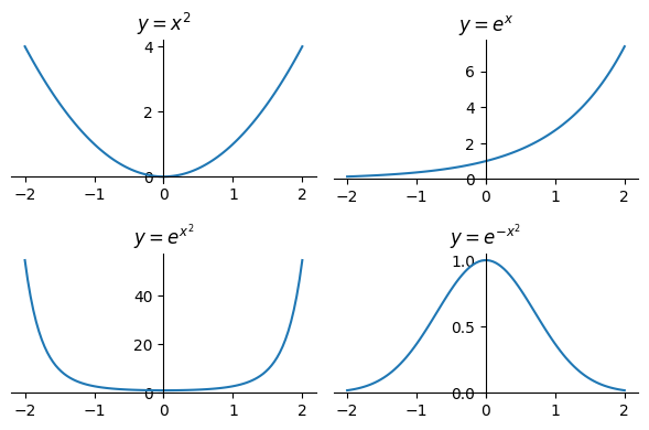
Our function is supposed to be a PDF, so it should integrate to one. $$ \int_{-\infty}^{\infty} f(x)\,dx = 1 $$
Pulling the constant \(c\) out of the integral, we get the following constraint. $$ c \int_{-\infty}^{\infty} e^{-b^2 x^2}\,dx = 1 $$
Now we perform integration by substitution to simplify the integral \(\lparen \int f(u) \frac{du}{dx}\,dx = \int f(u)\,du \rparen\) . $$ u = bx, \quad du = b\,dx $$
After the substitution, the Gaussian integral \(\int_{-\infty}^{\infty} e^{-u^2}\,du\) appears, which evaluates to \(\sqrt{\pi}\). $$ \frac{c}{b} \int_{-\infty}^{\infty} e^{-u^2}\,du = 1, \quad \frac{c}{b} \sqrt{\pi} = 1 $$
Thus, we can get rid of one out of two unknowns by replacing \(b^2 = \pi c^2\) in our function. $$ f(x) = c \cdot e^{-\pi c^2 x^2} $$
This already is a bell-shaped probability density function, but the mean is zero and the variance is unknown at the moment (we will see below that the variance of the current function is \(\frac{1}{2\pi c^2}\)).
Restricting the family of bell-shaped functions to those that integrate to one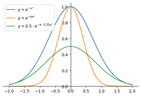
Alternatively, we could replace \(c = \frac{b}{\sqrt{\pi}}\) and actually this is the way in which Jaynes (2003) presents the derivation, but it doesn't really matter as we'll eventually arrive at the same formula.3
We would like to parameterize our function with the variance \(\sigma^2\). Since we have only one unknown or parameter left, our goal will be to express it in terms of the variance or standard deviation. We start with the definition of the variance. $$ \sigma^2 = \int_{-\infty}^{\infty} (x-\mu)^2 f(x)\,dx $$
Since \(\mu = 0\), expanding \(f(x)\) gives us the following equation (again, pulling the constant factor \(c\) out of the integral). $$ \sigma^2 = c \int_{-\infty}^{\infty} x^2 e^{-\pi c^2 x^2}\,dx $$
We find the integral via integration by parts \(\lparen \int u\,dv = uv - \int v\, du \rparen\). $$ u = x, \quad du = dx, \quad dv = x \cdot e^{-\pi c^2 x^2}\,dx $$
To continue our integration by parts we need the function \(v\), which we can find via integration by substitution (the "inside" function being substituted is \(-\pi c^2 x^2\)). $$ v = \frac{1}{- 2\pi c^2} e^{-\pi c^2 x^2} $$
Putting it all together, we get the variance in the form of the following subtraction. $$ \sigma^2 = c \Bigg[ \frac{x}{-2 \pi c^2} e^{-\pi c^2 x^2} \Bigg]_{-\infty}^{\infty} - c \int_{-\infty}^{\infty} \frac{1}{- 2\pi c^2} e^{-\pi c^2 x^2}\, dx $$
The first term is approaching zero for both limits because \(x\) is squared and multiplied with a negative constant in the exponent of a factor. If we look a bit closer at the second term, we find the normalized function \(f(x)\) in it, which, of course, integrates to one. $$ \sigma^2 = - \frac{1}{- 2\pi c^2} \int_{-\infty}^{\infty} c e^{-\pi c^2 x^2}\, dx = \frac{1}{2\pi c^2} $$
Now we solve for \(c\) and obtain this constant in terms of the standard deviation. $$ c = \frac{1}{\sigma \sqrt{2 \pi}} $$
Substituting this expression for \(c\) in \(f(x)\) yields the formula for bell-shaped PDFs with a mean of zero and a standard deviation of \(\sigma\). $$ f(x) = \frac{1}{\sigma \sqrt{2 \pi}} e^{\frac{-x^2}{2 \sigma^2}} $$
If we play with the parameter \(\sigma\), we see that it determines the inflection points of the curve around the center.
Controlling the standard deviation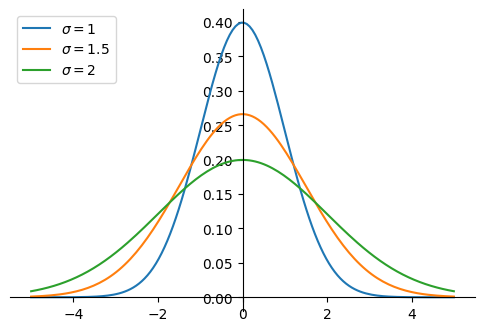
So far our function has a mean of zero. To obtain a function with mean \(\mu\), we simply shift the input \(x\) by \(-\mu\). $$ f(x) = \frac{1}{\sigma \sqrt{2\pi}} e^{-\frac{1}{2} \lparen \frac{x - \mu}{\sigma} \rparen^2} $$
For example, subtracting two from the input shifts the curve two to the right.
Shifting the input \(x\) by \(-\mu\)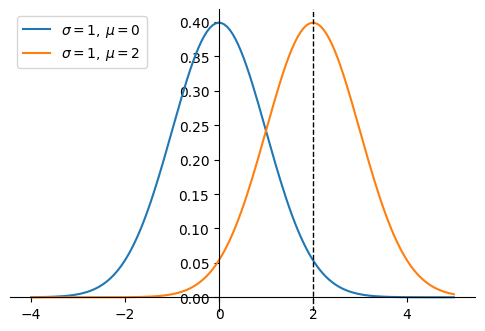
Thus, we finally arrived at the formula stated at the top of this page.
1 An archer or a darts player trying to hit the middle of a circular target are common variants.
2 Keep in mind that we are dealing with PDFs here, the derivatives of cumulative distribution functions. An event for which we can compute a probability is not a single value or point, but always a set of values (a real interval in one dimension or an area in two dimensions, which may be arbitrarily small). Since we are not so much interested in computing probabilities, but want to derive a PDF, I omit the infinitesimals for clarity.
3 If we replace \(c = \frac{b}{\sqrt{\pi}}\), we get \(f(x) = \frac{b}{\sqrt{\pi}} \cdot e^{-b^2 x^2}\), or \(f(x) = \sqrt{\frac{\alpha}{\pi}} \cdot e^{-\alpha x^2}\) with \(b = \sqrt{\alpha}\) and \(\alpha > 0\) (this is the form that Jaynes gives after normalization). This function has a variance of \(\sigma^2 = \frac{1}{2\alpha}\). If we solve for \(\alpha\) and substitute back into the equation, we get the same result as at the end of the variance section of this post. Interestingly, for \(\alpha = 1\), we get \(f(x) = \frac{e^{-x^2}}{\sqrt{\pi}}\), the standard normal distribution of Gauss and Laplace, whereas if we substitute \(c = 1\) in \(f(x) = c \cdot e^{-\pi c^2 x^2}\), we end up with the standard normal distribution of Stigler (1982) that has a variance of \(\sigma^2 = \frac{1}{2\pi}\).
Herschel, J. F. (1869). On the theory of probabilities. Journal of the Institute of Actuaries and Assurance Magazine, 15(3), 179-218.
Jaynes, E. T. (2003). Probability theory: The logic of science. Cambridge University Press.
Stigler, M. S. (1982). A Modest Proposal: A New Standard for the Normal. The American Statistician, 36(2), 137-138.
This page was moved from my old website.